In the wake of Apple’s announcement that they incorporating differential privacy in many of the Apple products, I think it’s high time to continue my quest to have a firm grasp on differential privacy. I wrote an introductory note on differential privacy in my old blog [1], but it was over 3 years ago. One could be forgiven in thinking that I should have become an expert by now. Yeah, no.

It was typical Apple not disclosing any information that would have justified the move as visionary, and that would also have satisfied many security researchers. There are two ways to see it, and they are not mutually exclusive. First, it’s testament to how the technology has matured that it would soon become the norm. Second, there are tremendous risks in adopting this technology without transparency, as it is teemed with non-technological trade-offs. The most important consideration is how to trade privacy for utility. Of course the fact that Apple even bring this consideration into a table is hugely encouraging, but this effort would be but all for nothing if they did not make their decisions public. It is essential for the users to understand the risks before sharing, and concealing them would completely offset the benefit of differential privacy.

Though papers on differentially private algorithms and mechanisms still fill me with dreads, I have started to comprehend and appreciate some of the very cool properties of differential privacy, thanks to two awesome lecture notes I found online [2, 3]. The rest of this article I will try to articulate these properties as much as I understand them.

Definition

Differential privacy is only applicable to randomized algorithm \(\cal{A}(\cal{D}) = \cal{Y}\) (\(\cal{Y}\) can be a probability space, hence the correct formula is \(\cal{A}(\cal{D}) \in \cal{Y}\)). It means applying \(\cal{A}\) on the same input will give different results, based on the whatever randomness embedded in \(\cal{A}\) (or its coin toss). It’s easy to image that \(\cal{D}\) is the database of \(n\) rows, and \(\cal{Y}\) is the space of vectorized results \(\langle y_1, y_2, .., y_m \rangle\).

Ideal privacy. We want \(\cal{A}(.)\) to not reveal information about a given individual \(x\), given arbitrary auxiliary information. This means publishing the result of \(\cal{A}\) does not violate any privacy. This, however, is impossible to achieve. A counter example is that \(x\) is an associate professor, and \(\cal{A}(.)\) on the database of university staff reveals that an average salary of an associate professor is (approximately) \(100K\). Thus, we know that \(x\) salary is \(100K\) in average — new information being revealed as the result is published.

Relaxed (differential) privacy. The ideal privacy is impossible, meaning that performing an analysis task on the data inevitably leads to leakage. Differential privacy attempts to relax the requirement in order to beat the impossibility result. It requires analysis result to be almost the same whether \(x\) is in \(\cal{D}\) or not. It means that \(x\) can opt out of the analysis without affecting the result. It also means that \(x\)’s privacy is not decreased if she is in \(\cal{D}\). Hence the name differential.

Formal definition. Algorithm \(\cal{A}: \mathbb{D} \to \mathbb{Y}\) is \(\epsilon\)-differentially private if for all \(\cal{Y} \in \mathbb{Y}\) and \(\cal{D}_1, \cal{D}_2 \in \mathbb{D}\) where \(\cal{D}_1\) and \(\cal{D}_2\) differs by at most 1 entry, then:

\[\frac{Pr[{\cal A}({\cal D}_1) = {\cal Y}]}{Pr[{\cal A}({\cal D}_2) = {\cal Y}]} \leq e^\epsilon \qquad \quad (1)\]

Different notations. Equation \((1)\) can be expanded or re-written as in the following ways:

• When \(\epsilon\) is small, \(e^\epsilon \approx 1+x\). Thus:

\[1 - \epsilon \leq \frac{Pr[{\cal A}({\cal D}_1) = {\cal Y}]}{Pr[{\cal A}({\cal D}_2) = {\cal Y}]} \leq 1 + \epsilon \qquad \quad (2)\]

• Because \(Pr[f(.) = y \;\vert\; X=x ] = Pr[f(x) = y]\), we have:

\[\frac{Pr[{\cal A}(.) = {\cal Y} \;\vert\; {\cal D} = \cal{D}_1]}{Pr[\cal{A}(.) = \cal{Y} \;\vert\; \cal{D} = \cal{D}_2]} \leq e^\epsilon \qquad \quad (3)\]

Differential privacy written in Equation (3) be stated as: the probably of \(\cal{A}(.)\) outputting the same value given the input \(\cal{D}_1\) is similar to that given the input \(\cal{D}_2\).

Privacy budget The value \(\epsilon\) is called privacy budget, which embodies the differences between two output distribution of the algorithm. This can be viewed as the amount of privacy violation allowed by the user, and the algorithm must work within this amount. Large budget means large differences between the two distribution is allowed. Strong level of differential privacy means small budget.

Security equivalence

The formal definition (Eq. 2) expresses the bound of leakage in information theoretic sense, which is useful in most statistical analysis. Most mathematicians or statisticians can work comfortably with this definition. For people coming from a security background like me, a definition based on a security game would be easier to grasp. And I was glad to finally find such a definition in [2]. It was truly refreshing seeing the same problem in a new light.

The game, as usual, involves a challenger (Alice) and an adversary Bob. It proceeds as follows:

1. Alice generates \({\cal D} = \langle x_1,x_2,..,x_n \rangle\).

2. Alice sends \(\cal{A}\), \({\cal D}' = \langle x_1,x_2,..,x_{n-1} \rangle\) and \(\cal{Y} = {\cal A}({\cal D})\) to Bob.

3. Bob guesses \(x_n\).

4. Bob wins if it can guess \(x_n\) correctly with a probability greater than a random guess.

The winning probability of Bob is the level of privacy decrease that \(x_n\) suffers, i.e. the advantage the adversary would have had in identifying \(x_n\) in the dataset. We can prove that if \(\cal{A}(.)\) is \(\epsilon\)-differentially private, the probability of Bob winning the above game is bound by \(\epsilon\).

For simplicity, let \(n=k=1\) and \(y = \cal{A}(x) \in \{0,1\}\) for \(x \in \{0,1\}\). Furthermore:

1. (A1) Alice chooses \(x\) by flipping an unbiased coin, i.e. \(Pr[x=0] = Pr[x=1] = \frac{1}{2}\).

2. (A2) \(Pr[{\cal A}({0}) = 0] > Pr[{\cal A}(1) = 0]\).

The best guessing strategy by Bob is maximum likelihood estimation, i.e.

\[guess \leftarrow argmax_j Pr[{\cal A}(j) = y] \qquad (4)\]

Combining Eq.4 with assumption A2 gives us \(guess = y\).

Thus:

\[\begin{align*} Pr[\text{Bob wins}] & = Pr[\text{guess}\ 0, x_n=0] + Pr[\text{guess}\ 1, x_n=1] \\ & = \frac{1}{2} Pr[\text{guess}\ 0 \,\vert\, x_n=0] + \frac{1}{2} Pr[\text{guess}\ 1 \,\vert\, x_n=1] \\ & = \frac{1}{2} Pr[y = 0 \,\vert\, x_n=0] + \frac{1}{2} Pr[y = 1 \,\vert\, x_n=1] \qquad \\ & = \frac{1}{2} Pr[{\cal A}(0) = 0] + \frac{1}{2} Pr [{\cal A}(1) = 1] \\ & = \frac{1}{2} + \frac{1}{2} (Pr[{\cal A}(0) = 0] - Pr [{\cal A}(1) = 0]) \\ & \leq \frac{1}{2} + \frac{\epsilon}{2} \qquad (5) \end{align*}\]

Eq.5 suggests that if \(\epsilon\) is small, so is the leakage. In particular, if \(\epsilon = neg(.)\) for a negligible function \(neg(.)\), the definition reduces to the indistinguishibility notion found in traditional cryptography. In practice, however, \(\epsilon\) is quite substantial (in the range of \((0.1, 10]\)) for the analysis to be useful. Thus, there is a real risk of decrease in privacy when an individual is included in the data.

Properties

The definition of differential privacy implies three key properties that are instrumental in designing differential private systems.

Sequential composition

When a differentially private algorithm (analysis) is run \(k\) times over the same dataset, the privacy deteriorates. The consequence is that if the analyst doesn’t want the privacy to get worse (and eventually lost), he should bound the number of runs. Publishing the result is a special case when the analysis is done once then the data is discarded.

Formally, let \({\cal A}_i\) for \(1 \leq i \leq k\) be independent \(\epsilon_i\)-differentially private algorithms. Then the algorithm \({\cal B}\) made up from a sequence of \({\cal A}_i\), i.e. \({\cal B} = ({\cal A}_1, .. {\cal A}_k)\) is \(\sum_i \epsilon_i\)-differentially private.

Proof. For any sequence of \(\langle {\cal Y}_1, {\cal Y}_2, .., {\cal Y}_k \rangle\), and \({\cal D}_1\) and \({\cal D}_2\) different by at most 1 entry, we have:

\[\begin{align*} Pr[{\cal B}({\cal D}_1) = {\cal Y}_k] & = Pr[{\cal A}_1({\cal D}_1) = {\cal Y}_1, .., {\cal A}_k({\cal D}_1)= {\cal Y}_k] \\ & = \prod_i Pr[{\cal A}_1({\cal D}_1) = {\cal Y}_1] \\ & = \prod_i e^{\epsilon_i}Pr[{\cal A}_i({\cal D}_2) = {\cal Y}_i] \\ & = e^{\sum_i \epsilon_i} \prod_i Pr[{\cal A}_i({\cal D}_2) = {\cal Y}_i] \\ & = e^{\sum_i \epsilon_i} Pr[{\cal B}({\cal D}_2) = {\cal Y}_k] \\ \end{align*}\]

Recall that \(\epsilon\) is called privacy budget, and the lower it is the better for privacy. An implication of composition is that every time you make a pass through the data with a \(\epsilon\)-differentially private algorithm, the overall privacy budget is decreased by \(\epsilon\). A common practice is to fix the budget \(\epsilon\) at the beginning and ration it out to sub-analyst tasks. For example, let \(\cal B\) be consists of a sum (\({\cal A}_1\)) and a product (\({\cal A}_2\)) operation over the data. Suppose the user wants differential privacy with budget \(\epsilon = 1\), then we can design \({\cal A}_1\) with budget \(\epsilon_1 = 0.2\) and \({\cal A}_2\) with budget \(\epsilon_2 = 0.8\). There is no privacy guarantee after running \(\cal B\). Once the budget is exhausted, discard the data.

Partitioning

Note that sequential composition property considers multiple algorithms computing over the entire dataset. When different algorithms touch different part of the data, then we have better bounds in terms of privacy budget. An example is the algorithm computing the histogram of the data, which is essentially a set of range count queries over disjoint ranges. More specifically, consider \(\cal D\) consisting of 2 fields: Smoker (Y/N) and Age (0..120). Then the histogram of the numbers of smokers for different ages can be constructed by executing count operations over range [0..10), [10,20),… The count operations touches different parts of \(\cal D\), i.e. removing one entry would change the result of only one query.

Formally, let \({\cal P}_1,.., {\cal P}_k\) be the partitions of the original data. Let \({\cal A}_1,..,{\cal A}_k\) be algorithms working on the corresponding partitions, and \({\cal A}_i\) is \(\epsilon_i\)-differentially private. Then the algorithm \({\cal B}({\cal D}) = {\cal Y} = ({\cal A}_1({\cal P}_1)={\cal Y}_1, .., {\cal A}_k({\cal P}_k)={\cal Y}_k)\) is \(max(\epsilon_i)\)-differentially private.

Proof. Consider \({\cal D}_1\) and \({\cal D}_2\) differing in at most 1 entry. Without loss of generality, assume the difference is in the first partition, i.e. \({\cal P}_1\) and \({\cal P'}_1\).

\[\begin{align*} Pr[{\cal B}({\cal D}_1) = {\cal Y}] & = \prod_i Pr[{\cal A}_i({\cal P}_i) = {\cal Y}_i]\\ & = e^{\epsilon_1} Pr[{\cal A}_1({\cal P}'_1) = {\cal Y}_1] \prod_{i > 1} Pr[{\cal A}_i({\cal P}_i) = {\cal Y}_i]\\ & = e^{\epsilon_1} Pr[{\cal B}({\cal D}_2) = Y]\\ & \leq e^{max(\epsilon_i)} Pr[{\cal B}({\cal D}_2) = Y]\\ \end{align*}\]

Histogram algorithm can be made differentially private with very low budget because it works on partitioned data. The budget is independent of the unit width. For example, if the count query is \(\epsilon\)-differentially private, any histogram producing either \(1\) bar or \(N\) bars are \(\epsilon\)-differentially private.

Post processing

How the result of a differentially private algorithm \(\cal A\) is used does not affect individual privacy. Note that this post processing — applying another algorithm on the result — is different to sequential composition of different algorithms. Post processing does not compute over the data, but sequential composition does.

Formally, let \(f: \mathbb{Y} \to \mathbb{V}\) be a post-processing function. If \({\cal A}: \mathbb{D} \to \mathbb{Y}\) is \(\epsilon\)-differentially private, then \(f({\cal A})\) is also \(\epsilon\)-differentially private.

Proof. For any \({\cal V} \in \mathbb{V}\), let \({\cal Y} \in {\cal Y}\) such that \(f(Y) = {\cal V}\). For any two \({\cal D}_1, {\cal D}_2\) differing in at most one entry:

\[\begin{align*} Pr[f({\cal A}({\cal D}_1)) = \cal{V}] & = Pr[{\cal A}({\cal D}_1) = {\cal Y}] \\ & = e^\epsilon Pr[{\cal A}({\cal D}_2) = {\cal Y}] \\ & = e^\epsilon Pr[f({\cal A}({\cal D}_2)) = {\cal V}] \\ \end{align*}\]

This property is significant to the practicality of differential privacy. It basically says that if you perform an analysis whose results can be reused in future analysis, user privacy is not affected by the future analysis. Thus the data can be safely thrown away. Take histogram as an example. Initial histogram computation may incur an \(\epsilon\) privacy budget. Once done, however, any useful function (arbitrary range count queries) can be done over the histogram without changing the initial privacy budget. A more complex example is linear regression [4], which publishes \(\epsilon\)-differentially private objective (loss) function. The process of optimizing the function is complex (SGD algorithm), but the final regression result will still preserve \(\epsilon\) differential privacy.

The key take away from this property is that: in designing a differential private mechanism, look for a simple pre-processing step that can be done with small privacy budget. It’s better to shift complexity to the post-processing step.

Group privacy

One minor property that I don’t want to leave out is group privacy. What happened when the data is changed by more than 1 entries. This makes sense in settings where data entries are related to each other, and removing one also removing the other.

The main result is that if the user want privacy for a group of rows, he must assign a bigger privacy budget, i.e. \(k\) times bigger for group of \(k\).

Formally, Let \({\cal A}\) be \(\epsilon\)-differentially private for two datasets differing in 1 entry, then \({\cal A}\) is \(k\epsilon\)-differentially private for two datasets differing in \(k\) entries.

Proof. Let \({\cal D}_1, .. {\cal D}_{k+1}\) be datasets in which \({\cal D}_1\) and \({\cal D}_{k+1}\) differ in \(k\) entries. Furthermore, \({\cal D}_i\) and \({\cal D}_{i+1}\) differs in 1 entry.

\[\begin{align*} Pr[{\cal A}({\cal D}_1) = Y] & = e^\epsilon Pr[{\cal A}({\cal D}_2) = Y] \\ & = e^{2\epsilon} Pr[{\cal A}({\cal D}_3) = Y] \\ & = ... \\ & = e^{k\epsilon} Pr[{\cal A}({\cal D}_{k+1}) = Y] \end{align*}\]

Mechanisms

The definition above states the conditions which a randomized algorithm \(\cal A\) must satisfy for it to be considered differentially private. Also, any differentially private algorithms will enjoy the three properties: sequential composition, partitioning and immune to post-processing. Here, I will discuss how to design such \(\cal A\) in practice. Given an algorithm \(A\), the goal is to transform it to a differentially private version \(\cal A\) with a privacy budget of \(\epsilon\). The transformation is done by adding carefully crafted noises to the output of \(\cal A\). So far, \(A\) is being restricted to classes of rather simple algorithms, for the main difficulty is to maximize the utility of \(\cal A\) for a fixed budget \(\epsilon\). I wouldn’t be too surprised if there is (or will be) an impossibility result claiming that there are certain classes of \(A\) not amenable to differential privacy.

In any analysis task, there are two steps: data collection and analysis. The second step can be repeated many times. In practice, there steps are combined in two different system models. In the first, there is a trusted party who collects the data and answers queries on a differentially private manner. In the second, no trusted party is assumed, thus the data collection process must be made differentially private. Note that in this case, all subsequent analysis on the collected data is differentially private (due to the post-processing property).

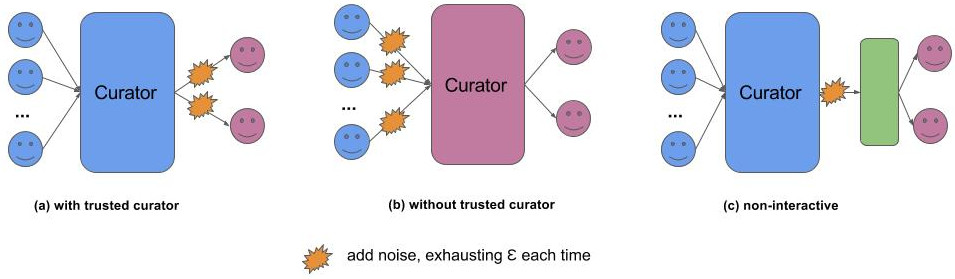
The figure shows three typical models for deploying differential privacy in practice. They differ mainly in which entities are considered trusted (blue), which leads to different places to enforce differential privacy.

No trusted curator

In this settings, data owners have to make sure their data is differentially private before sending it to the curator. The idea is to add noise in order to hide the true value.

Randomized response is an algorithm having been used by social scientists for very long time. Assume the data is a binary value (0 or 1). The algorithm \(\cal A\) proceeds as follows

1. Flip a coin. If it comes up head, answer the true value.
2. Else, flip another coin and answer Y if head and N if tail.

This algorithm is \(ln(3)\)-differentially private, for the following:

\[\frac{Pr[{\cal A}(1) = 1]}{Pr[{\cal A}(0) = 1]} = \frac{Pr[{\cal A}(0) = 0]}{Pr[{\cal A}(1) = 0]} = \frac{3/4}{1/4} = 3\]

The partitioning property can be applied here, to ensure that if all data owners follow the same algorithms, then the combined published data is \(ln(3)\)-differentially private. More important, the post-processing property is also applicable here. As a consequence, any subsequent analysis on the data procured by \(\cal A\) is \(ln(3)\)-differentially private. Note that the analysis must account for the error in the data: the probability of a randomized response returning the true value is only \(\frac{3}{4}\). One way to mitigate to lower the analysis error is to collect more and more data so that important patterns can eventually appear.

Google is employing this approach in their system called RAPPORT [5] which collects data from Chrome users about their settings and preferences. The main challenges addressed in RAPPORT is how to offset the error due to randomized response, for which the system uses hashing, Bloom filter and complex statistical techniques for the analysis. If I have to bet on what Apple is doing with differential privacy, with words like hashing being passed around, I’d go for the same approach like RAPPORT. But one caveat is that RAPPORT aims for data which rarely changes or changes very slowly. How would Apple modify it for fast-changing data like philological, locational data will be interesting to see.

Trusted curator

Although randomized response is intuitive and can offer a reasonable amount of privacy, its major drawback is poor utility (only 75% chance of a published value being the true one). Thus, the analyst (curator) will have to work with inaccurate data. By trusting a curator in not leaking the data and only computing differentially private function, the analyst can get more accurate results.

Interactive vs. non-interactive. Interaction between the curator and analyst can be interactive (a) or non-interactive (c). In the former, the curator exposes an interface to which the analyst can issue queries. Like a database, the curator takes a query, computes and returns the result. This approach, however, is limited by the sequential composition property. In particular, each query consumes a certain amount of the overall privacy budget. Suppose the user only allows for a budget of \(\epsilon\), and there are \(Q\) queries (count, sum, average, etc.), for each query the curator must perform a \(\epsilon_i\)-differentially private algorithm such that \(\sum_i \epsilon_i \leq \epsilon\). When another query comes and there an \(\epsilon_r > 0\) left, the curator can refuse the query, or accept it and perform the query with tight budget (which often lead to highly inaccurate result).

Designing an interactive system like the above is highly complex, as it involves managing the budget and perhaps predicting the future queries. A more interesting approach is to leverage the post-processing property of differential privacy: the curator publish a single representative function of the data, like histogram. Unlike the interactive case, there is only one operation over the data, hence the privacy budget can be fixed to a very low value. A function like histogram can output very useful result to be used by other queries (range queries, counts, etc.). A majority of papers I read on differentially privacy algorithm focus on this non-interactive settings. There is even a framework, called DPBench, for benchmarking these different non-interactive algorithms [6].

Laplace noises For a numerical algorithm \(A\), the most common method to make it differentially private is to add noises drawn from a zero-centered Laplace distribution.

More formally, let \(\Delta = max\vert\vert A({\cal D}_1) - A({\cal D}_2) \vert\vert_1\) be the global sensitivity of \(A\). \(\delta\) represents the maximum change \(A\)’s output when the data is changed by one item. Let \({\cal A}({\cal D}) = A({\cal D}) + Laplace(\frac{\Delta}{\epsilon})\) where the Laplace distribution has \(0\) mean. Then the algorithm \(\cal A\) is \(\epsilon\)-differentially private.

The proof for this can be found on Wikipedia. For some algorithms, like count and average, this mechanism introduces noises not too large for the outputs to be useful. Lots of research effort have been trying to minimize the overall noise by means of minimizing \(\delta\).

Complex algorithms Note that Laplace method is applicable to numerical algorithms. Many other algorithms do not output simple numbers. For example, machine learning algorithms produce models which are often sets of parameters in a complex, non-convex function. One way to make them differentially private is to add noise to the model parameters. But reasoning how much noise to be added is hugely challenging, because the parameter sensitivity to the input/training data is difficult to analyse. Another way is to make the objective function differentially private, as opposed to the model itself. In fact, the model essentially estimates the objective function’s local minima. The process of training the model (SGD) then can be considered as post-processing step and therefore omitted in the privacy analysis. This is a huge reduction in complexity, but the remaining step of making the objective function differentially private is by no means trivial.

As a consequence, state-of-the-art studies in differentially private machine learning are restricted to a simple set of machine learning models: linear classifier, decision tree, regression, etc. As deep learning is rapidly becoming the norm, differential privacy for deep learning models could become the new focus of the field, especially considering how much data needed for training the models.

[1] https://anhdinhdotme.wordpress.com/2013/03/26/on-differential-privacy/

[2] https://www.acsu.buffalo.edu/~gaboardi/teaching/cse711Spring2016/Lecture1.pdf

[3] http://people.eecs.berkeley.edu/~sltu/writeups/6885-lec20-b.pdf

[4] http://vldb.org/pvldb/vol5/p1364_junzhang_vldb2012.pdf

[5] http://static.googleusercontent.com/media/research.google.com/en//pubs/archive/42852.pdf

[6] https://arxiv.org/pdf/1512.04817.pdf