2019 started with a bang at work. My school organized a research week with a series of distinguished research talks delivered by world-class researchers. I hardly came away from any talk without learning anything new or interesting. The first day covered distributed systems, in glorious theoretical depth and practical complexity. Having only recently gotten less scared of this field, I left Valerie King’s presentation with wholly new understanding of the FLP theorem. Which is to say that my previous, though unstated, view of the theorem was wrong. Well, not as much wrong as incomplete. And that prompted me re-reading some papers, then spent several days wrestling with the original FLP paper. This blog is intended to capture what I understood so far. Knowing how subtle distributed systems are, it will not be the last on FLP and consensus protocols.

FLP and its implication

At a high level, FLP theorem says that consensus in an asynchronous network is impossible in the presence of node failure. This holds even for a single crash failure. We are reminded that crash failure is the most simple form of failure in distributed systems. The FLP result, as my initial understanding goes, has this implication:

In practical terms, we cannot simultaneously have safety (all non-faulty nodes agrees/decides on the same value) and liveness (the protocol terminates with a decision). Therefore, every consensus protocol must either sacrifice one property, or relax assumption about network asynchrony.

Most state-of-the-art consensus protocols follow the second strategy. PBFT, for example, assumes partially synchronous networks in which there exists an unknown bound on message delivery. PBFT achieves safety even in fully asynchronous network condition, and liveness under period of synchrony, as permitted by FLP.

So far, this view of FLP is not wrong. But it is not the whole truth. What I’ve been missing is that

FLP concerns only deterministic consensus protocols.

(This fact is stated so clearly in the original paper that I have only myself to blame for my initial, shallow understanding of one of the most important results in computer science.)

Now before I go and repent for this gross oversight, it is worth mentioning that I did sense something amiss when reading Andrew Miller’s HoneyBadger protocol (HBFT) which claims to work in an asynchronous systems. Having failed to understand all its details, I drew a conclusion that HBFT circumvented FLP by sacrificing safety: it achieves agreement only probabilistically. Well, now that was wrong!

A deterministic consensus protocol, as properly defined in FLP, means that nodes in the protocol behave deterministically. Determinism is a property of of node behavior, not of the final outcome. More specially, a node output (its decision) is entirely determined by the sequence of input events the node receives. All protocols that I had so far known of are deterministic. PBFT, Raft and Paxos, for examples, contains no randomness. When they receives a message, there path of execution is completely deterministic. Of course, different orders of inputs lead to different paths; but again that mapping of sequence of input to execution (and subsequently to output) is completely deterministic.

Non-deterministic protocol

So what does a non-deterministic consensus protocol looks like. Well, opposite of a deterministic thing is a randomized (or probabilistic) thing. A randomized algorithm’s output depends not only on its external input, but also on a random coin which is flipped during its execution. So, given two exactly the same inputs, the algorithm may output two different values.

FLP theorem does not apply to randomized protocol. Viewed this way, it is a positive result, giving researchers another way to engineer practical consensus protocols. There are only a small numbers of such algorithms, the most famous one is by Ben-Or in 1983, and they all share the same structure as follows:

• Each node has a source of randomness. Some algorithms allow the node to have its private, local coin; other optimize for cases when there exists a global coin. All algorithms proceed in many rounds of voting.

• Each node broadcasts its value to the network, and waits for \(n-f\) messages to come back. This constitutes a round of execution, after which the node moves on to another round. Note that it cannot wait for more than \(n-f\) messages, due to network asynchrony.

• There are some thresholds \(t\) defined in \(n\) and \(f\). If the node receives more than \(t\) messages with the same value, it can decide immediately.

• There are some other threshold \(t'\), below which the node tosses the coin and vote for that random value in the next round.

The probability that a node will decide at round \(r\) is of this form

\[P = 1 - (1-x)^r\]

which means \(P=1\) as \(r \to \infty\). State-of-the arts randomized protocols compete with each other by lowering the expected number of rounds by which the nodes decide. Many trade fault tolerance (the ratio of \(t\) against \(n\)) for constant and low expected number of round.

Why would it work? One direct question to ask is why, intuitively, non-determinism helps circumventing FLP. The core idea here is that in asynchronous networks, we assume the worst, that is the adversary has total control over message delivery with the only constraint that it will eventually deliver messages. In deterministic settings, sequence of messages is extremely important. In fact, the adversary in FLP craftily delay messages so that the nodes can never decide. In contrasts, the effect of message delivery (and order) is less important in non-deterministic setting, because the node behavior is also dependent on some randomness that the adversary cannot control. In other words, the adversary exerts less power in this setting, and therefore cannot always prevent the algorithm from reaching agreement.

---

FLP model

Now let us formally describe FLP. As many classic distributed systems papers, FLP is deceptively short and sweet. But only by re-reading it so many times, together with working backwards, that I am able to feel how the proof works.

The node

Each node is fully specified by its state and a transition function. The state consists of the input value, the output value (starting with a default value \(b\)), and any temporary variables during execution. The transition function is the meat. It is invoked by a receiving a message from the network:

• Given the message and current state as input, it deterministically moves the node to a new state.
• It may send many messages to the network during execution of the transition function.

The network

Nodes communicate through the network which is modeled as a centralized buffer. Controlled by the adversary, it consists of messages exchanged between node. A message is of the form \((p,m)\) where \(p\) is the message destination, \(m\) is the content.

An asynchronous network is characterized by the fact that the adversary controls when a message is delivered. In particular, the adversary can reorder messages in the buffer and insert arbitrary number of empty (or null) messages to the buffer. For instance, instead of delivering a message \((p,m)\) to \(p\), the adversary can simply deliver \((p,\emptyset)\). In either case, \(p\)’s transition function is invoked. The real message \(m\) can be delayed for arbitrarily long.

However, delayed messages is not the same as lost messages. The asynchronous network does provide a form of reliability: over infinite period of time, \((p,m)\) will eventually be delivered. More specifically, if \(p\) infinitely asks the buffer for a message, and there exists a \((p,m)\) in the buffer, \(p\) will receive it. The problem here is the word infinity, which in this case means there is no bound on the delay. In contrast, in partially synchronous settings, there is an unknown, yet finite period after which \((p,m)\) is delivered.

Terminologies

A configuration C comprises states of all the nodes in the system, plus the message buffer. At any given time, \(C\) represent the system’s global states. At a configuration \(C\), any node may take a step by receiving a message \(e\) from the network, then execute its transition function, thereby changing its state and consequently move the system to a new configuration \(C'\). We say that \(C'\) is the result of applying \(e\) to \(C\), written as \(e(C) = C'\).

An initial configuration is a configuration where the buffer is empty and every node is in its initial, fresh state. Every consensus protocol starts from an initial configuration.

A schedule, or run consists of a sequence of steps \(\langle .., (p_i, m_i), ..\rangle\). Such a sequence can be of infinite length, since there can be an infinite number of \((p, \emptyset)\) in the buffer. A schedule \(\sigma\) can be applied to a configuration \(C\) (which is not necessarily an initial configuration), by iteratively applying events in \(\sigma\) to \(C\). For example, \(\sigma=\langle e_1, e_2, e_3 \rangle\), then \(\sigma(C) = e_1(e_2(e_3(C)))\).

A configuration \(C\) is accessible for a protocol \(P\), if there exists an initial configuration \(C_0\) and a schedule \(\sigma\) such that \(\sigma(C_0) = C\).

####Concerning safety A configuration \(C\) has a decision value \(v\) if there exists \(p \in C\) such that \(p\) output value is \(v\). Another way to say it is that \(C\) decides on \(v\). Note that \(C\) may have more than one decision values. But we are only concerned with valid (or safe) protocol \(P\) such that:

Every accessible configurations has only 1 decision value. And for all \(v \in \{0,1\}\) there exists an accessible configuration with that value.

This definition of validity is in fact weaker than what we commonly require for consensus. Here, it only needs some nodes to reach a decision, whereas ordinary consensus is valid only if all non-faulty nodes reach a decision. Nevertheless, if it can be proven that this weaker version is impossible, there is no hope for the stronger version.

Concerning liveness

A deciding run is a schedule whose final configuration has a decision value. Recall again that we are only dealing with valid deciding runs, in which the configuration has only one decision value.

A configuration \(C\) is bivalent if there exists two deciding runs \(\sigma_0, \sigma_1\) that lead to configurations with decision values \(0\) and \(1\) respectively. \(C\) is \(0\)-valent (or \(1\)-valent) if all reachable configurations by deciding runs have decision value of \(0\) (or \(1\) respectively). In layman term, a bivalent configuration is one in which the protocol can go both way, i.e. there exists an important event that flips the decision one way or another. Once such event occurs, the protocol enters an univalent state which it can never goes back. Consider \(e(C) = C'\).

• If \(C\) is bivalent, \(C'\) can be either bivalent or univalent.

• If \(C\) is \(i\)-valent, \(C'\) is also \(i\)-valent.

A non-faulty node is one that all messages sent to it will be delivered, whereas a faulty node stops receiving messages at some point. What interesting is that we can define faulty behavior through the message buffer:

• If a node is not faulty, it infinitely asks for messages and the buffer will eventually deliver.
• Otherwise, the message buffer stops delivering messages to the faulty node.

An admissible run is a schedule in which there is at most one faulty node. Let \(\sigma\) be a schedule. If \(p\) is not faulty, all messages \((p,m)\) entered the buffer will appear in the sequence. If \(p\) is faulty, there is a point in \(\sigma\) after which no event \((p,m)\) is delivered.

Putting it together

A correct consensus protocol under one faulty node is one in which every admissible run is a deciding run. And no such protocol exists.

Here we have the familiar definition of consensus protocol: validity (deciding run) and termination (admissible run).

---

FLP proof

The proof of FLP is quite layered. But each layer is short and sweet. Together they remind me of an old saying that in mathematics and science, short theorems accompanied by short proofs are often the most beautiful and the most impactful.

The proof is based on contradiction. By assuming that a correct consensus protocol \(P\) exists, we are going to build up a number of lemmas which are put together to derive contradiction. I am going to highlight these lemmas’ core ideas and some subtlety that I struggled with.

1. Lemma 1 (diamond property): from a starting configuration \(C\), if two schedule \(\sigma_0, \sigma_1\) does not have any node in common (if \((p,m) \in \sigma_0\), there is no message delivered to \(p \in \sigma_1\), then \(C' = \sigma_0(\sigma_1(C)) = \sigma_1(\sigma_0(C))\). In other words, two disjoint schedules can be applied commutatively to a configuration. This is true because one message affects only the node that receives it, and because the configuration is merely an aggregation of all nodes’ states.

2. Lemma 2 (starting at a bivalent configuration): if \(P\) exists, then there exists a bivalent initial configuration. The implication here is that one can start \(P\) from a point at which the decision is not yet determined, meaning that the final decision is dependent not only on the starting inputs, but also the behavior of the message buffer. The proof goes like this: assume the contrary, that is all initial configurations of \(P\) are univalent.

   • One requirement for correctness is that there exists two different, accessible configurations that decides on \(0\) and on \(1\) respectively. And because \(i\)-valent configuration can only lead to configurations that decide \(i\), there must exists two initial configuration \(I_0\) and \(I_1\) that are \(0\)- and \(1\)-valent respectively.

   • Consider an initial configuration \(I\) which is \(0\)-valent. By changing the starting value of one node, we get an adjacent configuration \(I'\) which is also an initial configuration. Let assume again that \(I'\) is \(0\)-valent. By applying a chain of such transformation (changing starting value of the nodes, one at a time) we can any other initial configurations from \(I\). One of such reachable configurations must be \(1\)-valent. Therefore, there exists two initial configurations \(I_0\) and \(I_1\) differing only in the starting value of one node \(p\), and they are \(0\)- and \(1\)-valent respectively.

   • Consider \(I_0\) and an admissible run \(\sigma\) in which \(p\) is faulty. This is allowed because \(P\) can tolerate one fault, which may as well be \(p\). And \(P\) being correct means \(\sigma\) is a deciding run. It must therefore decide on \(0\). Now apply \(\sigma\) to \(I_1\). By Lemma 1 this should lead to the same configuration as with \(I_0\), which decides on \(0\). But this is not possible, since \(I_1\) is \(1\)-valent.

   So it means there exists a bivalent initial configuration.

3. Lemma 3 (maintaining bivalent configuration): if \(P\) exists, given a bivalent configuration \(C\), let \(e=(p,m)\) be an event applicable to \(C\). We delay \(e\), then apply it to every reachable configurations from \(C\) to get a set of configurations \(D\). \(D\) is the result of applying \(e\) last, and it contains a bivalent configuration. The implication here is that the adversary, being able to control the order of message delivery, can guide the system from one bivalent configuration to another configuration. The proof is again by contradiction: assume that \(D\) does not contain bivalent configurations.

   • \(D\) contains both \(0\)- and \(1\)-valent configuration. The reasoning for this is quite straightforward in the paper so I’ll ignore it here.

   

   • There exist two neighboring configurations reachable from \(C\) such that applying \(e\) to them results in a \(0\)- and \(1\)-valent configurations in \(D\). More specifically, there exists \(C_0, C_1\) reachable from \(C\) and \(e'=(p',m')\) such that \(C_1 = e'(C_0)\) or \(C_0 = e'(C_1)\), \(D = e(C_0)\) is \(0\)-valent and \(D'=e(C_1)\) is \(1\)-valent. The paper states that this fact can be derived via “easy” induction, which I find anything but.

     First, \(C_0\) and \(C_1\) are not necessarily \(0\)- and \(1\)-valent. Recall that an \(i\)-valent configuration can be reached directly in two ways: from an \(i\)-valent or a bivalent configuration.

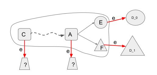
     Second, let us find such two neighbors \(C_0\) and \(C_1\), keeping in mind that any bivalent configuration reachable from \(C\) must become univalent after applying \(e\) (due to the contradiction assumption). Recall that \(C\) is bivalent, hence there is a path to another bivalent configuration \(A\) after which there can only be univalent configurations (see the Figure above). Extending \(E\) and \(F\) with \(e\) will lead to a \(0\)- and \(1\)-valent configurations in \(D\). Now let us consider \(A'=e(A)\). Because \(A' \in D\), it must be univalent (remember the contradiction assumption). If \(A'\) is \(0\)-valent, then we can assign \(C_0 \leftarrow A\) and \(C_1 \leftarrow F\). Otherwise, \(C_0 \leftarrow E\) and \(C_1 \leftarrow A\).

   • Without loss of generality, let \(e'=(p',m')\) and \(C_1 = e'(C_0)\). There are two further cases: 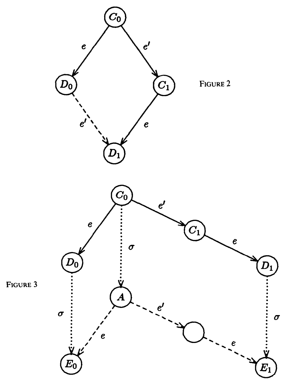Figure 2 and 3 from the original paper

     • If \(p \neq p'\) (Figure 2), then \(e(e'(C_0)) = e'(e(C_0))\) thanks to the diamond lemma. But this means \(D_0\) leads to both \(0\) and \(1\), violating the assumption of non-bivalency in \(D\).

     • If \(p == p'\) (Figure 3), then there exists a deciding run \(\sigma\) in which \(p\) is faulty. I spent two days trying to show why \(\sigma\) exists. Under the assumption that \(P\) exists, we only need to show that \(\sigma\) is a part of an admissible run by \(P\) (remember, correctness of \(P\) means every admissible run is a deciding run). Let’s say \(C_0 = \sigma'(I)\) for some initial state \(I\). The question becomes whether there exists \(\sigma\) in which \(p\) makes no step, and \(\langle \sigma', \sigma\rangle\) is an admissible run.

       Yes. The adversary can construct \(\sigma\) based on \(\sigma'\) as follows. It stops delivering all messages destined for \(p\), and makes sure all messages for \(p' \neq p\) are delivered. The resulting schedule \(S = \langle \sigma', \sigma \rangle\) meet the definition for an admissible run. My original struggle with this lemma was because I thought if \(\sigma'\) contains one faulty node different to \(p\), then \(\sigma\) cannot be constructed. However, the liberating insight here is that even if \(p'\) appears as faulty in \(\sigma'\), we can make it non-faulty again in \(\sigma\) by delivering all of its messages. The only important trace is \(S\), which is admissible because all except \(p\) got all of their messages.

       Let us continue. Now that \(\sigma\) exists, applying the diamond lemma again lead us to contradiction. If \(A\) decides on \(0\), it can be moved to a state that decides on \(1\), meaning that two nodes decide two different values. Hence, \(P\)’s validity is violated. The same argument applies if \(A\) decides on \(1\).

The final proof

With Lemma 2 and 3, we are going to construct an admissible run that does not decide, which contradicts the assumption that \(P\) exists. The algorithm goes like this:

1. Start with a bivalent initial configuration \(C_0\), which exists by Lemma 2.
2. Choose a message \(e=(p,m)\) for node \(p\) which is at the head of a node queue \(Q\) (the queue starts out in random order). Find a run from \(C_0\) that ends with \(e\) at a bivalence configuration \(C_1\). Such a run exists because of Lemma 3.
3. Set \(C_0 \leftarrow C_1\), put \(p\) to the back of \(Q\), and repeat step 2.

This algorithm has an admissible run because after infinite steps all messages are delivered. But it never decides on any value, contradicting the assumption that every admissible run is a deciding run (or \(P\) terminates). QED.